This tutorial walks you through exactly how to create a neural network, line by line. We’ll start from zero and build the script incrementally so you understand why each part exists and how it works. By the end, you’ll have the full working code and the knowledge to modify it.
Prerequisites (Do these first)
Install Python (if you don’t have it): Download from python.org (version 3.8 or newer).
Setup project structure (open your terminal/command prompt and run):
mkdir python-neuralnet
cd python-neuralnet
python -m venv venv
# OR
# python3 -m venv venv

# Activate:
#   macOS/Linux → source venv/bin/activate
#   Windows    → venv\Scripts\activate
Install the required libraries (open your terminal/command prompt and run):
pip install pandas numpy matplotlib scikit-learnDownload the MNIST test dataset (mnist_test.csv):
- Easiest option: Direct download → https://python-course.eu/data/mnist/mnist_test.csv
- Alternative (very popular): Kaggle dataset “MNIST in CSV” → https://github.com/phoebetronic/mnist (download the mnist_test.csv file).
- Save the file in the same folder where you will create your Python script (or note the full path).
Format reminder: The CSV has no header. First column = digit label (0–9), next 784 columns = pixel values (0–255) for a 28×28 image.
Recommended environment: Use VS Code with a .py file.
Task 1: Read and Display Data
You are given a list of MNIST digit data, where each entry is a list containing a label (digit 0–9) as the first element, followed by 784 pixel values (28×28 image). Write a Python function that:
- Accepts this list of MNIST data as input.
- For each digit (0–9), finds up to 3 different images of that digit.
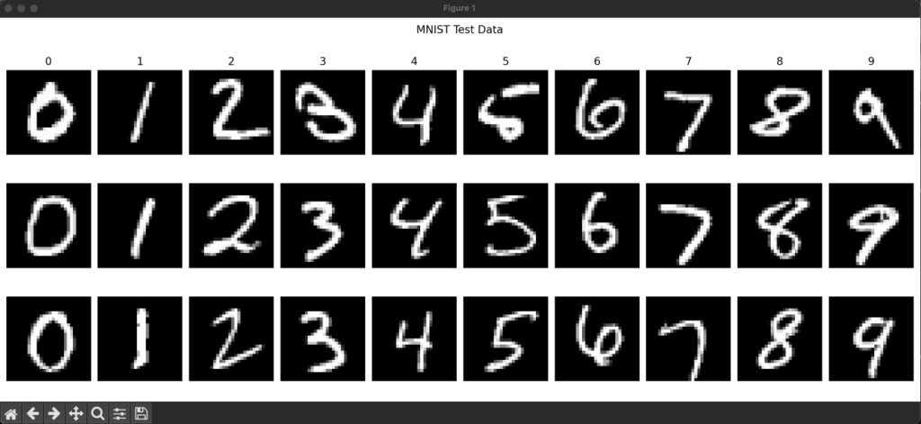
- Plots these images in a grid with 3 rows and 10 columns, where each column corresponds to a digit (0–9) and each row shows a different instance.
- The plot should not display axis ticks, and each column should be titled with the corresponding digit.
- The function should accept an optional title parameter to display as the figure title.
Include example usage in a main section that loads a CSV file into the required datalist format and visualizes it using your function. Expected result output:
Solution Task 1: Read and Display Data
1. Imports
# Import pandas for data manipulation
import pandas as pd
# Import numpy for numerical operations
import numpy as np
# Import matplotlib for plotting images
import matplotlib.pyplot as plt- pandas is used to read the CSV file easily.
- numpy is used to reshape the flat pixel arrays into 28×28 images.
- matplotlib.pyplot is used to create and show the figure with subplots.
2. The main function: visualize_datalist
def visualize_datalist(
    datalist, instances_per_digit=3, digits=range(10), title=None
):
This function takes a list of data rows (each row = [label, pixel1, pixel2, …, pixel784]) and creates a nice grid visualization.
2.1 Collecting the images we want to show
    # Create a dictionary to collect up to instances_per_digit for each digit
    instances = {digit: [] for digit in digits}

    # Iterate over all rows in the datalist
    for row in datalist:
        label = row[0]                    # first element is the digit (0-9)
        if label in instances and len(instances[label]) < instances_per_digit:
            instances[label].append(row[1:])   # keep the 784 pixel values

        # Stop early once we have enough images for every digit
        if all(len(v) == instances_per_digit for v in instances.values()):
break- It builds a dictionary instances where the keys are digits (0–9) and the values are lists of pixel rows.
- It stops as soon as it has collected the requested number of examples for every digit (early stopping = faster).
2.2 Creating the grid of subplots
    # Create the figure and axes
    fig, axis = plt.subplots(
        instances_per_digit, len(digits),
        figsize=(2 * len(digits), 2 * instances_per_digit)
    )

    if title:
fig.suptitle(title)- Creates a grid with instances_per_digit rows and 10 columns (one column per digit).
- The figsize makes each image roughly square and the whole figure readable.
2.3 Filling the grid with images
    # For each digit (column)
    for col, digit in enumerate(digits):
        # For each instance (row)
        for row in range(instances_per_digit):
            # Select the correct subplot (handles the case when there's only 1 row)
            ax = axis[row, col] if instances_per_digit > 1 else axis[col]

            if row < len(instances[digit]):
                # Convert flat list of 784 pixels → 28×28 image
                image = np.array(instances[digit][row]).reshape(28, 28)
                ax.imshow(image, cmap='gray')          # show in grayscale
                if row == 0:
                    ax.set_title(f"{digit}")           # label the column
            else:
                ax.axis('off')                         # hide empty slots

ax.axis('off') # remove ticks and borders for a clean look- Loops over columns (digits) and rows (instances).
- reshape(28, 28) turns the 784 pixel values into the original square image shape.
- imshow(…, cmap=’gray’) displays the handwritten digit.
- The first row of each column gets the digit number as a title.
2.4 Final touches
plt.tight_layout()   # prevents overlapping titles/axes
plt.show()           # displays the figure
3. Example usage (runs when you execute the file directly)
if __name__ == "__main__":
    # Path to the MNIST CSV data file
    path = r"mnist_test.csv"

    # Read the CSV file into a pandas DataFrame
    df = pd.read_csv(path, header=None)

    # Convert the DataFrame to a list of lists
    datalist = df.values.tolist()

    # Visualize the datalist
    visualize_datalist(datalist)
What happens here:
- Reads mnist_test.csv (no header row, so header=None).
- Converts the DataFrame to a plain Python list of lists (datalist).
- Calls visualize_datalist with default settings: 3 images per digit, digits 0–9, no extra title.
That’s it! The code is clean, efficient (stops early), and produces a clean visualization of MNIST digits straight from the raw CSV format.
Full Final Code (Copy-Paste Ready)
# Import pandas for data manipulation
import pandas as pd
# Import numpy for numerical operations
import numpy as np
# Import matplotlib for plotting images
import matplotlib.pyplot as plt

def visualize_mnist_datalist(
    datalist, instances_per_digit=3, digits=range(10), title=None
):
    """
    Visualize instances_per_digit images for each digit in datalist.
    Args:
        datalist (list): List of data rows, each row with label as first element and 784 pixel values.
        instances_per_digit (int): Number of images to show per digit.
        digits (iterable): Digits to visualize (default: 0-9).
        title (str or None): Title for the figure (default: None).
    """
    # Create a dictionary to collect up to instances_per_digit for each digit
    instances = {digit: [] for digit in digits}
    # Iterate over all rows in the datalist
    for row in datalist:
        # The first element is the label (digit)
        label = row[0]
        # Add the image data if we need more instances for this digit
        if label in instances and len(instances[label]) < instances_per_digit:
            instances[label].append(row[1:])
        # Stop if we have enough instances for all digits
        if all(len(v) == instances_per_digit for v in instances.values()):
            break
    # Create the figure and axes
    fig, axis = plt.subplots(
        instances_per_digit, len(digits),
        figsize=(2 * len(digits), 2 * instances_per_digit)
    )
    # Set the figure title if provided
    if title:
        fig.suptitle(title)
    # For each digit (column)
    for col, digit in enumerate(digits):
        # For each instance (row)
        for row in range(instances_per_digit):
            # Select the correct subplot
            ax = axis[row, col] if instances_per_digit > 1 else axis[col]
            if row < len(instances[digit]):
                # Convert the image data to a 28x28 array
                image = np.array(instances[digit][row]).reshape(28, 28)
                # Show the image in grayscale
                ax.imshow(image, cmap='gray')
                # Set the column title to the digit
                if row == 0:
                    ax.set_title(f"{digit}")
            else:
                # Hide the axis if no image
                ax.axis('off')
            # Hide axis ticks
            ax.axis('off')
    # Adjust layout to prevent overlap
    plt.tight_layout()
    # Display the plot
    plt.show()

# Example usage:
if __name__ == "__main__":
    # Path to the MNIST CSV data file
    path = r"mnist_test.csv"
    # Read the CSV file into a pandas DataFrame
    df = pd.read_csv(path, header=None)
    # Convert the DataFrame to a list of lists
    datalist = df.values.tolist()
    # Visualize the datalist
    visualize_mnist_datalist(datalist)
How to run it
- Save the code in a .py file (e.g. show_data.py).
- Make sure mnist_test.csv is in the same folder.
- Run the script → you should see a beautiful 3×9 grid showing three examples of each digit 0–9.
python show_data.pyNext-level customizations you can try:
- Change range
- Increase to 5 examples: change 3 everywhere to 5 and plt.subplots(5, 9, …).
- Add color: cmap=’viridis’ or any other matplotlib colormap.
Task 2: Prepare Data
You are given a CSV file containing MNIST digit data, where each row starts with a label (the digit) followed by 784 pixel values (28×28 image). Write a Python module that:
- Includes a main section that uses the visualization function from task 1 to display a sample of the training and test data, with appropriate figure titles.
- Reads the CSV file into a suitable data structure.
- Randomly splits the data into 80% training and 20% test sets.
- Normalizes the pixel values to the range [0.01, 0.99].
- Returns the training data, test data, training labels, and test labels as numpy arrays.
Solution Task 2: Prepare Data
1. Imports
import numpy as np
import pandas as pd
from sklearn.model_selection import train_test_split- numpy: For array operations and normalization.
- pandas: To easily read the CSV file.
- train_test_split: From scikit-learn to split the data into training and testing sets.
2. Main Function: load_and_prepare_data()
def load_and_prepare_data(path):
    """
    Reads, splits, and normalizes the MNIST data.
    Returns: (training_data, test_data, training_labels, test_labels)
    """
Step 2.1 – Reading the CSV
    df = pd.read_csv(path, header=None)
datalist = df.values.tolist()- Reads the CSV file (no header row).
- Converts it to a Python list of lists (same format as the previous script).
Step 2.2 – Separating Labels and Pixels
label_list = [row[0] for row in datalist]      # First column = digit (0-9)
data_list   = [row[1:] for row in datalist]    # Remaining 784 columns = pixels
Step 2.3 – Train / Test Split (80% / 20%)
    training_data, test_data, training_labels, test_labels = train_test_split(
        np.array(data_list),      # features (pixels)
        np.array(label_list),     # targets (labels)
        test_size=0.2,            # 20% for testing
        random_state=42,          # for reproducibility
        shuffle=True              # shuffle before splitting
)- Converts lists to numpy arrays first (required by train_test_split).
- Returns four arrays: training pixels, test pixels, training labels, test labels.
Step 2.4 – Normalization
    # Normalize to range [0.01, 1.0] instead of [0, 1]
    training_data = np.asarray(training_data) / 255 * 0.98 + 0.01
    test_data     = np.asarray(test_data)     / 255 * 0.98 + 0.01
Why this specific normalization?
- Original pixels are 0–255.
- Dividing by 255 gives 0.0–1.0.
- Multiplying by 0.98 and adding 0.01 shifts it to 0.01–0.99
- This is a common trick when training neural networks (especially those using sigmoid activation) to avoid extreme values (0 and 1) that can cause problems with some activation functions.
3. Example Usage (when running the script directly)
if __name__ == "__main__":
    # Import visualization function from another file
    from show_data import visualize_datalist

    # Load and prepare the data
    training_data, test_data, training_labels, test_labels = load_and_prepare_data(
        "mnist_test.csv"
    )
Reconstructing datalist format for visualization
    # Combine labels and normalized data back into original format
    training_datalist = [
        [int(label)] + list(vec)
        for label, vec in zip(training_labels, training_data)
    ]

    test_datalist = [
        [int(label)] + list(vec)
        for label, vec in zip(test_labels, test_data)
]- The visualize_datalist function (from the previous script) expects data in the original format: [label, pixel1, pixel2, …, pixel784].
- So we rebuild that structure using the split and normalized data.
Visualizing both sets
    print("Displaying training data samples:")
    visualize_datalist(training_datalist, title="Training")

    print("Displaying test data samples:")
    visualize_datalist(test_datalist, title="Test")
This will show two separate figures:
- Another grid with test examples (title: “Test”)
- One grid with training examples (title: “Training”)
Task 3: Define the Neural Network Signal Propagation
You are tasked with implementing the forward pass of a simple feedforward neural network for digit classification. The network has:
- 784 input nodes (one for each pixel of a 28×28 image)
- A configurable number of hidden nodes
- 10 output nodes (one for each digit 0–9)
Write a Python module that:
- Implements the sigmoid activation function.
- Implements a function test(input_vector, w_input_hidden, w_hidden_output) that:
- Accepts a flattened input vector, a weight matrix for the input-to-hidden layer, and a weight matrix for the hidden-to-output layer.
- Performs the forward pass using the sigmoid activation function for both layers.
- Returns the output vector.
- Includes a main section that:
- Initializes the weight matrices with random values between -0.5 and 0.5, using 200 hidden nodes.
- Loads test data using a function from the prepare data task.
- Runs the test function on the first test example and prints the output vector, the predicted label (index of the maximum output), and the true label.
Solution Task 3: Signal Propagation
1. Imports and Sigmoid Activation
import numpy as np

def sigmoid(x):
    """
    Compute the sigmoid activation for the input x.
    """
return 1 / (1 + np.exp(-x))- np is used for efficient array/matrix operations.
- sigmoid(x) is the activation function. It squashes any real number into the range (0, 1), which is useful for outputting probabilities in classification.
2. Forward Pass Function (test)
def test(input_vector, w_input_hidden, w_hidden_output):
    """
    Propagate input through the network.
    """
    # Reshape input to column vector
    x = input_vector.reshape(-1, 1)

    # Hidden layer
    hidden_inputs = np.dot(w_input_hidden, x)
    hidden_outputs = sigmoid(hidden_inputs)

    # Output layer
    final_inputs = np.dot(w_hidden_output, hidden_outputs)
    final_outputs = sigmoid(final_inputs)

    return final_outputs.flatten()
Step-by-step breakdown:
- input_vector.reshape(-1, 1) Converts the flat input (e.g., 784 pixels) into a column vector (shape (784, 1)), required for matrix multiplication.
- Hidden layer calculation:
- np.dot(w_input_hidden, x) → weighted sum of inputs
- Apply sigmoid() to get activations
- Output layer calculation:
- Same process: weighted sum → sigmoid
- .flatten() returns a 1D array (shape (10,)) with probabilities for each digit (0–9).
This is a two-layer network (input → hidden → output) with no bias terms.
3. Main Execution Block
if __name__ == "__main__":
    from prepare_data import load_and_prepare_data

    np.random.seed(40)                    # Reproducibility

    # Network architecture
    input_nodes = 784      # 28x28 pixels
    hidden_nodes = 200
    output_nodes = 10      # Digits 0-9

    # Random weight initialization
    w_input_hidden = np.random.uniform(-0.5, 0.5, (hidden_nodes, input_nodes))
w_hidden_output = np.random.uniform(-0.5, 0.5, (output_nodes, hidden_nodes))- Loads data from an external module (prepare_data.py).
- Creates weight matrices with random values in [-0.5, 0.5].
- Shape of w_input_hidden: (200, 784)
- Shape of w_hidden_output: (10, 200)
4. Testing on One Example
    # Load test data
    _, test_data, _, test_labels = load_and_prepare_data("mnist_test.csv")

    # Take first test sample
    first_test_input = test_data[0]
    first_test_label = int(test_labels[0])

    # Run forward pass
    output_vector = test(first_test_input, w_input_hidden, w_hidden_output)

    print("Output vector for the first test element:")
    print(output_vector)
    print("Predicted label:", np.argmax(output_vector))
    print("True label:", first_test_label)
What happens:
- Loads MNIST test set (images + labels).
- Runs the untrained network on the first image.
- np.argmax(output_vector) picks the digit with the highest output value (winner-takes-all).
Summary: Network Architecture
| Layer | Nodes | Activation | Purpose |
|---|---|---|---|
| Input | 784 | – | Flattened 28×28 image |
| Hidden | 200 | Sigmoid | Feature extraction |
| Output | 10 | Sigmoid | Probability per digit (0-9) |
Note: This network is randomly initialized and not trained, so the prediction will be essentially random (accuracy ≈ 10%). This is typically the starting point before implementing backpropagation.
Full Final Code (Copy-Paste Ready)
# Import numpy for numerical operations
import numpy as np

# Sigmoid activation function
def sigmoid(x):
    """
    Compute the sigmoid activation for the input x.
    """
    return 1 / (1 + np.exp(-x))

# Forward pass through the neural network
def test(input_vector, w_input_hidden, w_hidden_output):
    """
    Propagate input through the network.
    Args:
        input_vector (np.ndarray): Input vector
        w_input_hidden (np.ndarray): Weights from input to hidden layer
        w_hidden_output (np.ndarray): Weights from hidden to output layer
    Returns:
        np.ndarray: Output vector from the network
    """
    # Reshape input to column vector
    x = input_vector.reshape(-1, 1)
    # Calculate signals into hidden layer
    hidden_inputs = np.dot(w_input_hidden, x)
    # Apply sigmoid activation to hidden layer
    hidden_outputs = sigmoid(hidden_inputs)
    # Calculate signals into output layer
    final_inputs = np.dot(w_hidden_output, hidden_outputs)
    # Apply sigmoid activation to output layer
    final_outputs = sigmoid(final_inputs)
    # Return as 1D numpy array
    return final_outputs.flatten()

if __name__ == "__main__":
    # Import the data preparation function
    from prepare_data import load_and_prepare_data
    # Set random seed for reproducibility
    np.random.seed(40)
    # Network parameters
    input_nodes = 784
    hidden_nodes = 200
    output_nodes = 10
    # Initialize weight matrices with random values between -0.5 and 0.5
    w_input_hidden = np.random.uniform(
        -0.5, 0.5, (hidden_nodes, input_nodes)
    )
    w_hidden_output = np.random.uniform(
        -0.5, 0.5, (output_nodes, hidden_nodes)
    )
    # Load and prepare data
    _, test_data, _, test_labels = load_and_prepare_data("mnist_test.csv")
    # Test the network on the first test example
    first_test_input = test_data[0]
    first_test_label = int(test_labels[0])
    output_vector = test(first_test_input, w_input_hidden, w_hidden_output)
    print("Output vector for the first test element:")
    print(output_vector)
    print("Predicted label:", np.argmax(output_vector))
    print("True label:", first_test_label)
How to run it
- Save the code in a .py file (e.g. neural_net.py).
- Make sure mnist_test.csv is in the same folder.
- Run the script.
python neural_net.pyTask 4: Neural Network Training
You are tasked with implementing the training step for a simple neural network for digit classification. The network has:
- 784 input nodes (one for each pixel of a 28×28 image)
- 200 hidden nodes
- 10 output nodes (one for each digit 0–9)
Write a Python module that:
- Implements a function train(input_vector, label, w_input_hidden, w_hidden_output, learning_rate) that:
- Accepts an input vector, the correct label (0–9), a weight matrix for the input-to-hidden layer, a weight matrix for the hidden-to-output layer, and a learning rate.
- Performs a forward pass using the sigmoid activation function for both layers.
- Computes the error at the output and hidden layers.
- Updates the weights using the backpropagation algorithm and returns the updated weights.
- Includes a main section that:
- Initializes the weight matrices with random values between -0.5 and 0.5.
- Creates a random input vector and label.
- Prints the first 10 weights of each matrix before and after a single training step.
Solution Task 4: Network Training
1. Imports
import numpy as np
from neural_net import sigmoid- numpy for all matrix operations.
- sigmoid is a custom activation function (assumed to be 1 / (1 + exp(-x))).
2. The train() Function (Core Logic)
def train(input_vector, label, w_input_hidden, w_hidden_output, learning_rate):Purpose: Perform one step of stochastic gradient descent (backpropagation) on a single training example.
Step-by-step breakdown:
a) Prepare input
x = input_vector.reshape(-1, 1) # Shape: (784, 1) column vectorb) Forward pass – Hidden layer
hidden_inputs = np.dot(w_input_hidden, x)      # (200, 784) @ (784, 1) → (200, 1)
hidden_outputs = sigmoid(hidden_inputs)
c) Forward pass – Output layer
final_inputs = np.dot(w_hidden_output, hidden_outputs)   # (10, 200) @ (200, 1) → (10, 1)
final_outputs = sigmoid(final_inputs)
d) Create target vector (one-hot style)
targets = np.zeros((10, 1)) + 0.01          # All outputs start at 0.01
targets[label] = 0.99                       # Correct class = 0.99
e) Backpropagation – Calculate errors
output_errors = targets - final_outputs                    # How wrong was the output?

hidden_errors = np.dot(w_hidden_output.T, output_errors)   # Propagate error back to hidden layer
f) Update weights (Gradient Descent)
Output layer weights:
w_hidden_output += learning_rate * np.dot(
    (output_errors * final_outputs * (1.0 - final_outputs)),   # sigmoid derivative
    hidden_outputs.T
)
Hidden layer weights:
w_input_hidden += learning_rate * np.dot(
    (hidden_errors * hidden_outputs * (1.0 - hidden_outputs)),  # sigmoid derivative
    x.T
)
This is the classic backpropagation update rule for sigmoid activation:
- output * (1 – output) = derivative of sigmoid
- We add the adjustment (learning_rate × gradient)
Returns the updated weight matrices.
3. Main Block – Demonstration
if __name__ == "__main__":
    np.random.seed(42)

    # Network architecture
    input_nodes = 784      # 28x28 image flattened
    hidden_nodes = 200
    output_nodes = 10      # digits 0-9
    learning_rate = 0.2
Weight initialization (important to avoid symmetry):
w_input_hidden = np.random.uniform(-0.5, 0.5, (hidden_nodes, input_nodes))
w_hidden_output = np.random.uniform(-0.5, 0.5, (output_nodes, hidden_nodes))
Create dummy data:
input_vector = np.random.rand(input_nodes)   # Random "image"
label = np.random.randint(0, 10)              # Random correct digit
Train once and show weight changes:
print("Before training:", w_input_hidden.flat[:10])
w_input_hidden, w_hidden_output = train(...)   # One training step
print("After training:", w_input_hidden.flat[:10])
Key Concepts Illustrated
- In-place updates: The function modifies and returns the weight matrices.
- Forward Propagation: Input → Hidden → Output using matrix multiplication + sigmoid.
- Target Encoding: 0.01 / 0.99 instead of 0/1 (helps sigmoid, which never truly reaches 0 or 1).
- Backpropagation: Error flows backward from output to hidden layer.
- Weight Updates: Using the gradient (error × activation × derivative).
Complete File (Copy & Paste Ready)
# Import numpy for numerical operations
import numpy as np
# Import sigmoid activation function from neural_net
from neural_net import sigmoid

def train(input_vector, label, w_input_hidden, w_hidden_output, learning_rate):
    """
    Train the neural network on a single example.
    Args:
        input_vector (np.ndarray): Input vector of shape (784,)
        label (int): The correct label (0-9)
        w_input_hidden (np.ndarray): Weights from input to hidden layer
        w_hidden_output (np.ndarray): Weights from hidden to output layer
        learning_rate (float): Learning rate for weight updates
    Returns:
        tuple: Updated (w_input_hidden, w_hidden_output)
    """
    # Reshape input to column vector
    x = input_vector.reshape(-1, 1)
    # Calculate signals into hidden layer
    hidden_inputs = np.dot(w_input_hidden, x)
    # Apply sigmoid activation to hidden layer
    hidden_outputs = sigmoid(hidden_inputs)
    # Calculate signals into output layer
    final_inputs = np.dot(w_hidden_output, hidden_outputs)
    # Apply sigmoid activation to output layer
    final_outputs = sigmoid(final_inputs)
    # Create target vector (0.99 for correct label, 0.01 for others)
    targets = np.zeros((10, 1)) + 0.01
    targets[label] = 0.99
    # Calculate output layer error
    output_errors = targets - final_outputs
    # Calculate hidden layer error
    hidden_errors = np.dot(w_hidden_output.T, output_errors)
    # Update weights for hidden-output layer
    w_hidden_output += learning_rate * np.dot(
        (output_errors * final_outputs * (1.0 - final_outputs)),
        hidden_outputs.T
    )
    # Update weights for input-hidden layer
    w_input_hidden += learning_rate * np.dot(
        (hidden_errors * hidden_outputs * (1.0 - hidden_outputs)),
        x.T
    )
    # Return updated weights
    return w_input_hidden, w_hidden_output

if __name__ == "__main__":
    # Set random seed for reproducibility
    np.random.seed(42)
    # Network parameters
    input_nodes = 784
    hidden_nodes = 200
    output_nodes = 10
    learning_rate = 0.2
    # Initialize weight matrices with random values between -0.5 and 0.5
    w_input_hidden = np.random.uniform(
        -0.5, 0.5, (hidden_nodes, input_nodes)
    )
    w_hidden_output = np.random.uniform(
        -0.5, 0.5, (output_nodes, hidden_nodes)
    )
    # Create a random input vector and label for demonstration
    input_vector = np.random.rand(input_nodes)
    label = np.random.randint(0, output_nodes)
    # Display first 10 weights before training
    print("First 10 weights (input-hidden) before training:")
    print(w_input_hidden.flat[:10])
    print("First 10 weights (hidden-output) before training:")
    print(w_hidden_output.flat[:10])
    # Train the network once
    w_input_hidden, w_hidden_output = train(
        input_vector, label, w_input_hidden, w_hidden_output, learning_rate
    )
    # Display first 10 weights after training
    print("First 10 weights (input-hidden) after training:")
    print(w_input_hidden.flat[:10])
    print("First 10 weights (hidden-output) after training:")
    print(w_hidden_output.flat[:10])
Task 5: Run the Neural Network
You are given a modular neural network implementation for digit classification, split across several files:
- prepare_data.py: Loads, splits, and normalizes MNIST data.
- neural_net.py: Contains the sigmoid activation and forward pass (test) function.
- train_net.py: Contains the training (backpropagation) function.
Write a Python script (run_net.py) that:
- Imports the necessary functions from the above modules.
- Initializes the network parameters (input, hidden, and output nodes, learning rate).
- Initializes the weight matrices with random values between -0.5 and 0.5.
- Loads and prepares the MNIST data using the provided function.
- Trains the network on the entire training set, updating the weights after each example.
- Tests the trained network on the first test example, printing the output vector, predicted label, and true label.
- Visualizes the first test image using matplotlib.
Solution Task 5: Run the Neural Network
1. Imports
import numpy as np
from prepare_data import load_and_prepare_data
from neural_net import test
from train_net import train
import matplotlib.pyplot as plt- numpy: Used for all matrix operations (weights, activations, etc.).
- Custom modules:
- prepare_data: Loads and preprocesses MNIST CSV data.
- train_net: Contains the train() function (forward + backward pass).
- neural_net: Contains the test() function (forward pass only).
- matplotlib: To visualize the digit.
2. Reproducibility
np.random.seed(42)Fixes the random number generator so you get the same results every time you run the script.
3. Network Architecture Parameters
input_nodes = 784      # 28x28 pixels = 784
hidden_nodes = 200
output_nodes = 10      # digits 0-9
learning_rate = 0.2
This defines a 784 → 200 → 10 network.
4. Weight Initialization
w_input_hidden = np.random.uniform(-0.5, 0.5, (hidden_nodes, input_nodes))
w_hidden_output = np.random.uniform(-0.5, 0.5, (output_nodes, hidden_nodes))- Weights are randomly initialized between -0.5 and 0.5.
- Shape of w_input_hidden: (200, 784) → each hidden neuron has 784 weights.
- Shape of w_hidden_output: (10, 200) → each output neuron has 200 weights.
5. Data Loading
training_data, test_data, training_labels, test_labels = load_and_prepare_data("mnist_test.csv")This function (defined elsewhere) typically:
- Reads the CSV.
- Normalizes pixel values (usually to [0.01, 0.99] or [0, 1]).
- One-hot encodes labels or keeps them as integers.
- Returns NumPy arrays.
6. Training Loop (Online Learning)
for i in range(len(training_data)):
    input_vector = training_data[i]
    label = int(training_labels[i])
    w_input_hidden, w_hidden_output = train(
        input_vector, label,
        w_input_hidden, w_hidden_output,
        learning_rate
)- This is stochastic gradient descent (one example at a time).
- For every training image:
- Forward pass.
- Calculate error (usually using one-hot target).
- Backpropagate to update both weight matrices.
- Note: Training on all examples once = 1 epoch. Here it’s just one pass.
7. Testing on One Example
first_test_input = test_data[0]
first_test_label = int(test_labels[0])
output_vector = test(first_test_input, w_input_hidden, w_hidden_output)

print("Output vector for the first test element:")
print(output_vector)
print("Predicted label:", np.argmax(output_vector))
print("True label:", first_test_label)- test() does a forward pass only and returns the 10 output activations (probabilities-like scores).
- np.argmax() picks the digit with the highest score.
Example output might look like:
Output vector: [0.01, 0.02, 0.95, 0.03, ...]
Predicted label: 2
True label: 2
8. Visualizing the Image
plt.imshow(first_test_input.reshape(28, 28), cmap='gray')
plt.title(f"True label: {first_test_label}")
plt.axis('off')
plt.show()
Reshapes the flat 784-element vector back into a 28×28 image and displays it in grayscale.
Complete File
import numpy as np
from prepare_data import load_and_prepare_data
from neural_net import test
from train_net import train
import matplotlib.pyplot as plt

# Set random seed for reproducibility
np.random.seed(42)

# Network parameters
input_nodes = 784
hidden_nodes = 200
output_nodes = 10
learning_rate = 0.2

# Initialize weight matrices
w_input_hidden = np.random.uniform(-0.5, 0.5, (hidden_nodes, input_nodes))
w_hidden_output = np.random.uniform(-0.5, 0.5, (output_nodes, hidden_nodes))

# Load and prepare data
training_data, test_data, training_labels, test_labels = load_and_prepare_data("mnist_test.csv")

# Training loop
for i in range(len(training_data)):
    input_vector = training_data[i]
    label = int(training_labels[i])
    w_input_hidden, w_hidden_output = train(input_vector, label, w_input_hidden, w_hidden_output, learning_rate)

# Test the network on the first test example
first_test_input = test_data[0]
first_test_label = int(test_labels[0])
output_vector = test(first_test_input, w_input_hidden, w_hidden_output)

print("Output vector for the first test element:")
print(output_vector)
print("Predicted label:", np.argmax(output_vector))
print("True label:", first_test_label)

# Display the first test image
plt.imshow(first_test_input.reshape(28, 28), cmap='gray')
plt.title(f"True label: {first_test_label}")
plt.axis('off')
plt.show()